About
multi-variant Gaussians.
Fisher has describe first this analysis with his Iris Data Set.
A Fisher's linear discriminant analysis or Gaussian LDA measures which centroid from each class is the closest. The distance calculation takes into account the covariance of the variables.
Prerequisites
Statistical Learning - Simple Linear Discriminant Analysis (LDA)
Steps
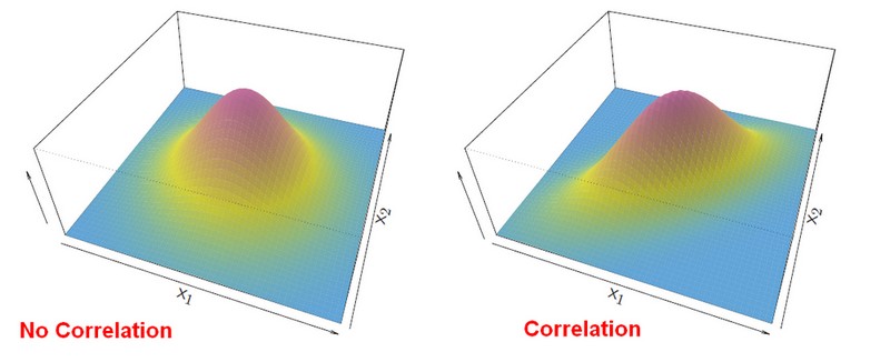
Density Function
Pictures of the Statistics - (Probability) Density Function (PDF) made with R:
Formulas:
<MATH> f(x)=\frac{1}{(2\pi)^{p/2}|\sum|^{1/2}} e^{\displaystyle - \frac{1}{2}(x-\mu)^T \sum ^{-1}(x-\mu) } </MATH>
This formula is just a generalization of the simple formula we had for a single variable. This is called a covariance matrix,
Discriminant Function
The discriminant functions is telling you how to classify.
The idea of the discriminant function is to compute one of these discriminant function for each of the classes, and then you classify it to the class for which it's largest. You pick the discriminant function that's largest.
If you go through the simplifications with linear algebra, you can do the cancellation and get the below formula:
<MATH> \delta_k(x) = x^T \sum ^{-1} \mu_k - \frac{1}{2} \mu^T_k \sum ^{-1} \mu_k + log \pi_k </MATH>
where:
- <math>x^T</math> is the transpose of the vector x containing all variables
- <math>\mu^T_k</math> is the transpose of the vector <math>\mu_k</math> containing all means
Despite its complex form it's still a linear function in x, where the coefficient is a vector.
Simplified form:
<MATH> \delta_k(x) = c_{k0} + c_{k1}x_1 + c_{k2}x_2 + c_{k3} x_3 + \dots + c_{kp} x_p </MATH>
where:
- x is not more a vector but an expansion of the previous vector expression. <math>c_{k1}x_1 + \dots + c_{kp} x_p = x^T \sum ^{-1} \mu_k</math>
- <math>c_{k0}= - \frac{1}{2} \mu^T_k \sum ^{-1} \mu_k + log \pi_k</math>
Probabilities
Once we have estimates <math>\delta_k(x)</math> , we can turn these into estimates for class probabilities:
<MATH> \hat{Pr}(Y=k|X=x) = \frac {\displaystyle e ^{\displaystyle \hat{\delta}_k(x)} } {\displaystyle \sum_{l=1}^K e ^{\displaystyle \hat{\delta}_l(x)}} </MATH>
Classification
So classifying to the largest <math>\hat{\delta}_k(x)</math> amounts to classifying to the class for which <math>\hat{Pr}(Y=k|X=x)</math> is largest.
When K = 2, we classify to class 2 if <math>\hat{Pr}(Y=k|X=x) >= 0.5</math> else to class 1.
Illustration
p = 2 and K = 3 classes
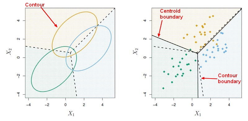
Here <math>\pi_1 = \pi_2 = \pi_3 = \frac{1}{3} </math> The dashed lines are known as the Bayes decision boundaries. Were they known, they would yield the fewest misclassification errors, among all possible classifiers.
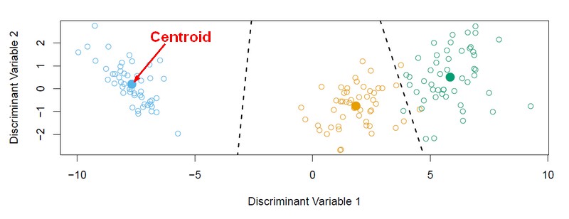
Discriminant Plot
When there are K classes, linear discriminant analysis can be viewed exactly in a K - 1 dimensional plot. Because it essentially classifies to the closest centroid, and they span a K - 1 dimensional plane. Even when K > 3, we can find the “best” 2-dimensional plane for visualizing the discriminant rule.
The three centroids actually line in a plane (a two-dimensional subspace), a subspace of the four-dimensional space and that's essentially the two-dimensional plot below that captures exactly what's important in terms of the classification.