About
Step functions, are another way of fitting non-linearities. (especially popular in epidemiology and biostatistics)
Articles Related
Procedure
Continuous variable are cut into discrete sub-ranges and fit a constant model in each of the regions. It's a piecewise constant (model|function).
Characteristics
Natural cut point
The piecewise constant functions are especially useful if they are some natural cut points that you want to use or/and are of interest.
Summary
what is the average income for somebody below the age of 35? You read it straight off the plot. This is often good food for summaries (in newspapers, reports, …)
Interaction
Useful way of creating interactions that are easy to interpret.
Example of interaction variable (between Year and Age) in a linear model:
X_1 = I(Year < 2005) . Age
X_2 = I(Year > 2005) . Age
where I is the R indicator function.
With this two variables, we will fit a different linear model as a function of age for the people who worked before 2005 and those after 2005. We will get two different linear functions in each age category. It's an easy way of seeing the effect of an interaction.
Local
One advantage over polynomial is that the calculation is local.
With polynomials, we have a single function for the whole range of the x variable. If I change a point on the left side, it could potentially change the fit on the right side for polynomials. But for step functions, a point only affects the fit in its partition and not the others.
Knots
Choice of cutpoints or knots can be problematic. For creating non-linearities, smoother alternatives such as splines are available.
Implementation
The function of the sub-ranges must be seen as binary variable.
Is x less than 35?
- If yes, you make it 1.
- If not, you make it a 0.
You creates then a series of dummy variables (zero-one variables) representing each group and you just fit those with the linear model.
Models
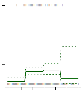
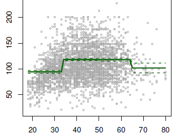
In the below plot, there is a cut:
- at 35
- at 50 (not really visible in the regression plot)
- and at 65.
<MATH> C_1(X) = I(X < 35); C_2(X) = I(35 \leq X < 50), \dots, C_3(X) = I(X \geq 65) </MATH>
Linear
Logistic