About
Although polynomials are easy to think of, splines are much better behaved and more local.
Articles Related
Procedure
With polynomial regression, you create new variables that are just transformations of the original variable.
And then just treat the problem as a multiple linear regression model with these new derived variables.
In these case, the coefficients are not really interesting whereas the (fitted|composed) functions at any particular value x0 is interesting (What does a new fitted function look like at a new value x0).
An extra variable is introduced to accommodate polynomials in the linear model:
- <math>{X}^n</math>
- with a coefficient regression <math>B_n</math>
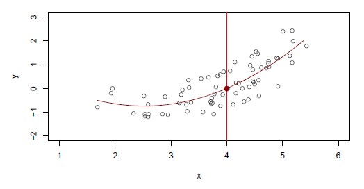
When the figure suggests that a polynomial regression may provide a better fit. <MATH> \begin{array}{rll} Y & = & B_0 + B_1 ( X ) + B_2 ( X_{2} ) + \dots + B_n ( X_{n} ) \\ Y & = & B_0 + B_1 ( X ) + B_2 ( {X}^2 ) + \dots + B_n ( {X}^n ) \\ \end{array} </MATH> where:
- The second extra variable will be from the second degree: <math>X_{2} = {X}^2</math>
- …
- The n extra variable will be from the n degree: <math>X_{n} = {X}^n</math>
That's a very easy way of allowing for non-linearities in a variable, and still use linear regression.
We still call it a linear model, because it's actually linear in the coefficients. But as a function of the variables, it's become non-linear.
It's linear in the coefficients but it's a non-linear function of x.
Characteristic
Tail behaviour
Polynomials regression have notorious tail behaviour that are very bad for extrapolation. Those tails tend to wiggle around. And you really wouldn't want to trust predictions beyond the range of the data or even to near the ends of the data.
Not local
Polynomial analysis is not local. With polynomial, the parameters affect the function everywhere and can have dramatic effect.
With polynomials, we have a single function for the whole range of the x variable. If I change a point on the left side, it could potentially change the fit on the right side.
Methods
Linear
Plot
It's a non-linear function that seems to capture what is going on in the data. where we see:
- the fitted function
- the pointwise standard error bands. The dotted bands that represents plus and minus 2 standard error.
Tail:
Notice that the standard error brands are wider at the ends as a result of what is called leverage. The data points thins out at the right end. (There is not so much data). There is less information for fitting the curve at the end and therefore the standard error gets wider. This effect is called wagging the tail of the dog. A polynomial is a very flexible function and is especially flexible at the end where the tails tend to wag around. That's what the standard error is indicating.
Variance
What is a variance of the fitted function at x0 ?
Since the fitted function is a linear function of the coefficients, we can get a simple expression for the pointwise variances. By using the covariance matrix of the fitted parameters, you can then get a simple expression, for the variance of this fitted value.
Pointwise means that the standard error band is pointwise. The band is showing at any given point what the standard error is. (not to be confused with global confidence bands)
What degree
The degree d is obviously a parameter (tuning parameter)
Often d is fixed at a small number (like two, three or four) else it can be selected by cross-validation.
Logistic
Logit Transform
<MATH> \begin{array}{rrrl} Pr(Y = 1|X) & = & p(X) & = & \frac{\displaystyle e^{\displaystyle B_0 + B_1 . X + \dots + B_n . X^n}}{\displaystyle 1+ e^{\displaystyle B_0 + B_1 . X + \dots + B_n . X^n}} \\ \end{array} </MATH>
Plot
A polynomial is used to fit a logistic regression.
The standard errors are at the end is pretty wide because it comes from the vertical scale that is pretty stretched (It's only ranging up to 0.2). With a scale from zero to one, it would look a lot more narrow.
- at the bottom of the plot all zeros occur (that are uniform across the range).
- above all the ones occur (most of them in the middle of the range and not many ones at the right end). There's so not enough data right at the end to estimate the function.
Confidence Interval
By getting the confidence intervals for the probabilities using direct methods, you might get outside of the range 0 and 1.
In order to overcome this situation, you compute upper and lower bounds on on the logit scale, and then inverse them through the logit transformations to get them on the probability scale. Those give you the confidence intervals for the fitted probabilities.
Quadratic
<math>\hat{Y} = \hat{f}(X) = \hat{B}_0 + \hat{B}_1 X + \hat{B}_2 X^2 </math>
where:
- Y is the target
- The hat <math>\hat{}</math> means estimated
- <math>B_0</math> to <math>B_n</math> are the regression coefficients
- X is the predictor
Using the Quadratic Model in place of Linear Model will decrease the Bias of your model.


