About
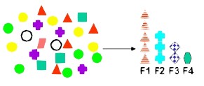
Feature extraction is the second class of methods for dimension reduction.
It's also sometimes known as dimension reduction but it's not.
It creates new attributes (features) using linear combinations of the (original|existing) attributes.
This function is useful for reducing the dimensionality of high-dimensional data. (ie you get less columns).
Applicable for:
- latent semantic analysis,
- data decomposition and projection,
- and pattern recognition.
We project the p predictors into a M-dimensional subspace, where M < p. This is achieved by computing M different linear combinations, or projections, of the variables. Then these M projections are used as predictors to fit a linear regression model by least squares.
Dimension reduction is a way of finding combinations of variables, extracting important combinations of variables, and then using those combinations as the features in regression.
Approaches:
- unsupervised: PCR, Principle Components Regression, (by far, the most famous dimension reduction)
- supervised: Partial least squares
Procedure
The idea is that by choosing wisely the linear_combinations (in particular, choosing the <math>\phi_{mj}</math> ), we will be able to beat ordinary least squares (OLS) with the raw predictors.
Linear Combinations
Let <math>Z_1, Z_2, \dots, Z_m</math> represent m linear combinations of the original p predictors (m<p).
<MATH> Z_m = \sum_{j=1}^p \phi_{mj} x_j </MATH>
where:
- <math>\phi_{mj}</math> is a constant
- <math>x_j</math> are the original predictors
(m<p) because if m equals p, dimension reduction will just give least squares on the raw data.
Model Fitting
Then the following linear model can be fitted using ordinary least squares:
<MATH> y_i = \theta_0 + \sum_{m=1}^M \theta_m z_{im} + \epsilon_i </MATH>
where:
- <math>i = 1, \dots, n</math>
This model can be thought of as a special case of the original linear regression model because (a little bit of algebra):
<MATH> \sum_{m=1}^M \theta_m z_{im} = \sum_{m=1}^M \theta_m ( \sum_{j=1}^p \phi_{mj} x_{ij} ) = \sum_{j=1}^p (\sum_{m=1}^M \theta_m \phi_{mj} ) x_{ij} = \sum_{j=1}^p \beta_j x_{ij} </MATH>
The latest term is just a linear combination of the original predictors (<math>x</math> ) where the linear combination involves <math>\beta_j</math>
<MATH> \beta_j = \sum_{m=1}^M \theta_m \phi_{mj} </MATH>
Dimension reduction fits a linear model through the definition of new <math>z</math> 's that's linear in the original <math>x</math> 's where the <math>\beta_j</math> 's need to take a very, very specific form.
In a way, it's similar to ridge and LASSO, it's still least squares, it's still a linear model in all the variables, but there's a constraint (penalty term) on the coefficients. We're not getting a constraint on the RSS amount but on the coefficient form <math>\beta_j</math> coefficients.
Dimension reduction goal wants to win the bias-variance trade-off by getting a simplified model with low bias and also low variance relative to a plain vanilla least squares on the original features.
Feature Extraction vs Ridge regression
Ridge regression is really different from dimension reduction methods (principal components regression and partial least squares) but it turns out that mathematically these ideas are all very closely related.
Principle components regression, for example, is just a discrete version of ridge regression.
Ridge regression is continuously shrinking variables, whereas principal components is doing it in a more choppy sort of way.
Algorithm
- Fourier
- Wavelet transforms
Example
Example of feature extractors:
- unigrams,
- bigrams,
- unigrams and bigrams,
- and unigrams with part of speech tags.
- Given demographic data about a set of customers, group the attributes into general characteristics of the customers

