About
John von Neumann invented merge sort in 1945. It requires O(n log n) comparisons.
A sorting algorithm for rearranging lists (or any other data structure that can only be accessed sequentially, e.g. file streams) into a specified order.
“Merge Sort” is an oldie but a goodie because it uses a divide an conquer stratgey.
Merge Sort is over 60, or maybe even 70 years old but it's still used all the time in practice, because this is one of the methods of choice for sorting.
Articles Related
The Sorting Problem
The sorting problem
- Input: array of n numbers, unsorted.
- Output: array of n numbers, sorted (from smallest to largest)
Assumption: numbers are distinct (with duplicates, the problem can even be easier)
Solution
The Merge Sort algorithm is a recursive algorithm.
It's a divide-and-conquer application, where we take the input array, we split it in half, we solve the left half recursively, we solve the right half recursively, and then we combine the results (you just walk pointers down each of the two sort of sub-arrays, copying over, populating the output array in the sorted order)

Pseudo-Code
- recursively sort 1st half of the input array
- recursively sort 2nd half of the input array
- merge two sorted sublists into one
Merge Pseudo code
Pseudo code for the Merge Code:
C = output array [length  =  n]
A = 1st sorted array [n/2]
B = 2nd sorted array [n/2]
i = 1
j = 1
for k = 1 to n
   if A(i) < B(j)
      C(k) = A(i)
      i++
   else [B(j) < A(i)]
      C(k) = B(j)
      j++
   end if
end for
Binary Tree
Merge sort by calling itself two times, create a binary tree.
A tree is said to be binary when it call itself two times.
Media ({{:algorithm:recursion_tree.svg?500}}). Error while rendering: The image (wiki://media>algorithm:recursion_tree.svg) does not exist
The merge sort binary tree has the following Properties:
Number of levels
- at the (outer|root) level, with an input size of <math>n</math>
- at level one, each of the first set of recursive calls operates on array of size <math>n/2</math> ,
- at level two, each array has size <math>n/4</math> ,
- … and so on until …
- at the base case, for merge sort the input array has a size one or less.
The number of levels of recursion is exactly the number of times we need to divide N by two, until we get down to a number that's most one and that's exactly the definition of a logarithm base two of n <math>log_2(n)</math>
The number of levels of the recursion tree is essentially logarithmic in the size of the input. The reason is basically that the input size is being decreased by a factor two with each level of the recursion.
The number of level the merge sort recursion tree have as a function of n (ie the leaves reside on the level) is then: <MATH>log_2(n)</MATH>
Number of function
At each level <math>j=0,1,2,... log_2(n)</math> , there are <math>2^j</math> subproblems, each of size <math>n/(2^j)</math>
Running Time
Running Time analysis.
There's a trade off between:
- on the one hand explosion of sub problems, a proliferation of subproblems
- and the fact that successive subproblems only have to solve smaller and smaller subproblems.
Merge Subroutine
The running time of the merge subroutine for an array of length n is:
- two initializations (i and j)
- n iterations with:
- 1 comparison (1.5)
- 1 assignment in the array C
- 1 incrementation of the counter (i or j)
- 1 incrementation of k
<MATH> \begin{array}{rrl} \text{Running Time} & <= & 4n + 2 \\ & <= & 6n \text{ (sinds n is always bigger than 1)} \end{array} </MATH>
Merge Sort
Outside of the recursive calls (The two recursive are not counted) merge sort does a single invocation of the merge subroutine. See Merge Sort binary tree properties to understand the number of level and work by level.
Work for the level <math>j</math>
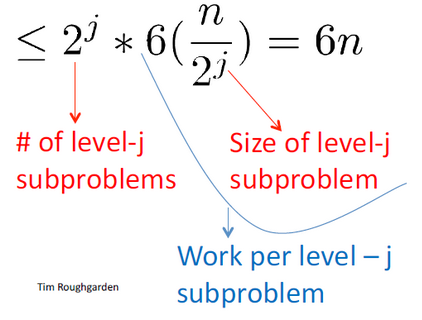
A remarkable cancellation happens on the <math>2^j</math> term that made the upper bound <math>6n</math> independent of the level <math>j</math> .
There is at most :
- at the root, six end operations ,
- at level one, at most six end operations,
- at level two,
- and so on.
The reason is a perfect equilibrium between two competing forces. First of all, the number of subproblems is doubling with each level of the recursion tree and secondly the amount of work that per sub-problem is halving with each level of the recursion tree's. Those two cancel out.
The upper bound 6n is then independent of the level j
Total
Total: Merge Sort requires then (as upper bound) in order to sort n numbers, the following numbers of operations:

<MATH> <= 6n.log_2n + 6n </MATH>
See Merge Sort binary tree properties to understand the number of level
Running Time Comparison <math>n.log_2(n)</math> vs <math>n^2</math>
log is running much, much, much slower than the identity function. And as a result, sorting algorithm which runs in time proportional to <math>n.log_2n</math> is much, much faster, especially as <math>n</math> grows large, than a sorting algorithm with a running time that's a constant times <math>n^2</math> .
Merge sort algorithm by using a divide an conquer stratgey has better performance than simpler sorting algorithms that scales with <math>n^2</math> like:
- Selection Sort (you do a number of passes through the way repeatedly, identifying the minimum of the elements that you haven't looked at yet)
- Insertion Sort
- and Bubble sorts (you identify adjacent pairs of elements which are out of order, … and then you do repeated swaps until in the end the array is completely sorted)
