Statistics - Piecewise polynomials
About
Piecewise polynomials generalize the idea of piecewise constants.
The idea try to get rid of the global polynomial because it's global and not local.
Instead of having a single polynomial over the whole domain of the variable, we fit different polynomials in each region (partition) instead of different constants.
The polynomials are fitted locally and has different level of continuity (smooth) throughout the whole range.
Articles Related
Formula
<MATH> y_i = \left\{ \begin{matrix} \beta_{10} + \beta_{11} x_i + \beta_{12} x_i^2 + \dots + \beta_{1n} x_i^n & \text{if } x_i < \href{knot}{knot} \\ \beta_{20} + \beta_{21} x_i + \beta_{22} x_i^2 + \dots + \beta_{2n} x_i^n & \text{if } x_i \geq \href{knot}{knot} \\ \end{matrix} \right. </MATH>
Continuity
The amount of continuity you can enforce, the order of continuity, is one less than the degree of the polynomial.
Splines are the maximum amount of continuity
Example
Non Continuous piecewise cubic
- Piecewise cubic polynomial in two regions. The knot is at 50.
They're two different cubic polynomials that just fit to the data with a break in the middle.
- The left one's fit to the data on the left.
- The right one's fit to the data on the right.
To suppress the break, it's better to add constraints to the polynomials, for example, continuity.
Continuous piecewise cubic
Two cubic polynomials (one in the left and one in the right) forced to be continuous at the knot.
In some situations, continuity alone is not enough (Notice the little kink in the middle) to have a smooth line. Continuity can then be enforced on the derivatives. See below.
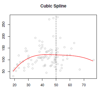
Cubic Spline
Cubic splines is a cubic polynomial in the left and the right and continuous at the knot.
There's the following constraints:
- The first derivatives continues at the knot,
- and the second derivatives continues at the knot.
We couldn't make the third derivative continuous, because then it would just be a global cubic polynomial. It's believed that a cubic spline, the discontinuity which exists in the third derivative is not detectable by the human eye.
The degree of continuity is 2 because it's a third degree polynomial.
Linear polynomials
A linear spline, or piecewise linear function has a degree zero continuity and is:
- linear in the left and the right.
- forced to be continuous at the knot.


