Statistics - Assumptions underlying correlation and regression analysis (Never trust summary statistics alone)
About
The magnitude of a correlation depends upon many factors, including:
- Random and representative sampling
- Measurement of X and Y:
- Validity of X and Y
- Several other assumptions:
- Normal distributions for X and Y
- Linear relationship between X and Y
Articles Related
Anscombe's quartet
In 1973, statistician Dr. Frank Anscombe developed a classic example to illustrate several of the assumptions underlying correlation and linear regression.
The below scatter-plots have the same correlation coefficient and thus the same regression line.
They have also the same mean and variance.
<MATH> Y = 3 + 0.5 X </MATH>
Only the first one on the upper left satisfies the assumptions underlying a:
- correlation analyses
- and a linear regression analyses

Datasaurus: Never trust summary statistics alone; always visualize your data
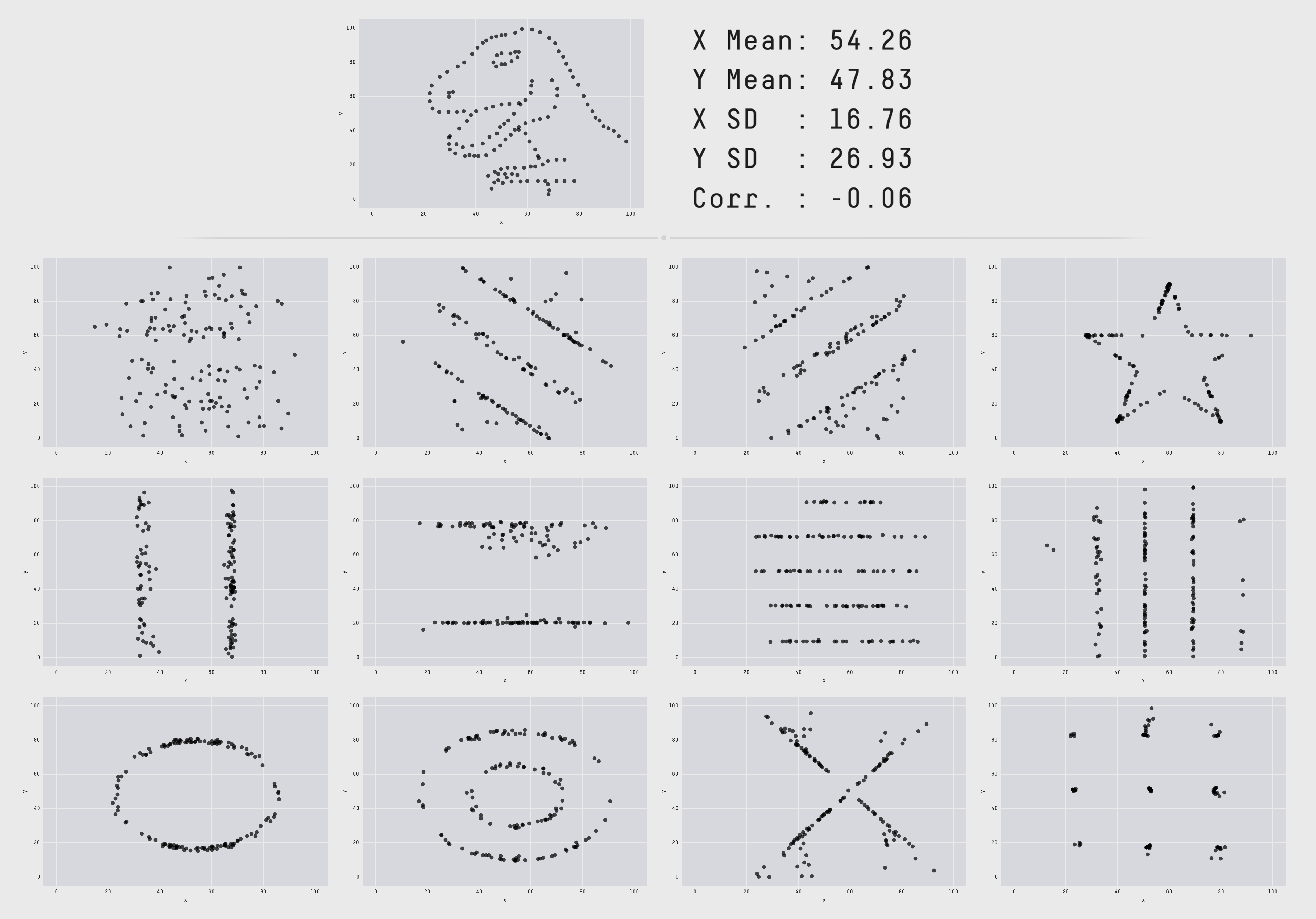
The Datasaurus Dozen. While different in appearance, each dataset has the same summary statistics (mean, standard deviation, and Pearson's correlation) to two decimal places.
See:
Bring your own doodles linear regression
Most of the examples of using linear regression just show a regression line with some dataset. it's much more fun to understand it by drawing data in. Bring your own doodles linear regression
How to
test the assumptions in a regression analysis ?
To test the assumptions in a regression analysis, we look a those residual as a function of the X productive variable. (X remaining on the X axis and the residuals coming on the Y axis).
For each of the individual, the residual can be calculated as the difference between the predicted score and a actual score.
If the assumptions are good, there must be:
- no relationship between X and the residual. They must be independent. The relation coefficient must be zero.
- some of the points above zero and some of them below zero. It will indicate Homoscedasticity