About
The average is a measure of center that statisticians call the mean.
To calculate the mean, you add all numbers and divide the total by the number of numbers (N).
<MATH> mean = \frac{\displaystyle \sum_{i=1}^{i=N}{x_i}}{N} </MATH>
The mean is not resistant.
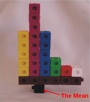
The mean is such an important measure of center because it is the numerical “balancing point” of the data set.
The mean is representative of the entire sample, if you don't have any skew or outliers effect.
Averaging is not an additive operation. You can’t average an average.
A sample mean represents a single point in a sampling distribution and is then an estimator.
The Will Rogers phenomenon is obtained when moving an element from one set to another set raises the average values of both sets. See Will Rogers phenomenon
Articles Related
Accuracy Statistic
Standard Error
The standard error for the mean is estimated from:
- the Sample Size (N)
- and the variance in the sample (Standard Deviation (SD))
under the assumption that the sample is random, normal and representative of the population.
<MATH> \text{Standard Error (SE)} = \frac{\href{Standard Deviation}{\text{Standard Deviation (SD)}}}{\sqrt{\href{Sample Size}{\text{Sample Size (N)}}}} </MATH>
The standard error increases then with an high variance (ie Standard deviation ) and a smallest sample size.
Example
Illustration of standard error calculation with R and the describe function (from the package psych)
require(psych)

describe(myData)
# se is the standard error for the mean
vars    n mean   sd median trimmed  mad   min  max range skew kurtosis   se
X1    1 1000 0.33 0.67   0.28    0.30 0.64 -0.81 1.85  2.66 0.44    -0.49 0.02
X2    2 1000 0.13 0.60   0.18    0.12 0.50 -1.18 1.77  2.94 0.17     0.31 0.02
y     3 1000 0.35 0.58   0.30    0.34 0.58 -0.75 2.04  2.79 0.42     0.18 0.02
# se = sd / sqrt(N)
descTable <- describe(myData)
descTable
myVariable.sd <- descTable[2,4]
myVariable.sd
myVariable.n <- descTable[2,2]
myVariable.n
myVariable.se <- descTable[2,4] / sqrt(descTable[2,2])
myVariable.se
myVariable.se == descTable[2,13]
TRUE
t-statistic
The t-value statistic is some observed value minus an expected value relative to standard error.
<MATH> \begin{array}{rrl} \text{t-value} & = & \frac{(\text{Observed} - \text{Expected})}{\href{Standard_Error}{\text{Standard Error}}} & \\ & = & \frac{(\href{Mean}{\text{Mean}} - 0)}{\href{Standard_Error}{\text{Standard Error}}} & \href{nhst}{\text{Playing the game of NHST the expected value is 0.}}\\ & = & \frac{\href{Mean}{\text{Mean}}}{\href{Standard_Error}{\text{Standard Error}}} & \\ \end{array} </MATH>
This t-statistics is the base of the t-test.
confidence interval
???